The forecast module#
EMHASS will need 4 forecasts to work properly:
PV power production forecast (internally based on the weather forecast and the characteristics of your PV plant). This is given in Watts.
Load power forecast: how much power your house will demand in the next 24 hours. This is given in Watts.
Load cost forecast: the price of the energy from the grid in the next 24 hours. This is given in currency/kWh.
PV production selling price forecast: the price at which you will sell your excess PV production in the next 24 hours. This is given in currency/kWh.
Some methods are generalized to the 4 forecasts needed. For all the forecasts it is possible to pass the data either as a passed list of values or by reading from a CSV file. With these methods, it is then possible to use data from external forecast providers.
Then there are the methods that are specific to each type of forecast and where the proposed forecast is treated and generated internally by this EMHASS forecast class.
For the weather forecast, the first method (open-meteo) uses Open-Meteo weather forecast API, which proposes detailed forecasts based on Lat/Lon locations. Another method (solcast) is using the Solcast PV production forecast service. A final method (solar.forecast) is using another external service: Solar.Forecast, for which just the nominal PV peak installed power should be provided. Search the forecast section on the documentation for examples of how to implement these different methods.
The get_power_from_weather method is proposed here to convert irradiance data to electrical power. The PVLib module is used to model the PV plant. A dedicated web app will help you search for your correct PV module and inverter: https://emhass-pvlib-database.streamlit.app/
The specific methods for the load forecast is a first method (typical) that uses historic values of a typical household power consumption. This method uses simple statistic methods and load power grouped by the same day-of-the-week of the current month. The load power is scaled using the parameter maximum_power_from_grid. A second method (naive) that uses a naive approach, also called persistence. It simply assumes that the forecast for
a future period will be equal to the observed values in a past period. The past period is controlled using the parameter delta_forecast_daily. A third method (mlforecaster)
uses an internal custom forecasting model using machine learning. There is a section in the documentation explaining how to use this method.
Note
This custom machine learning model is introduced from v0.4.0. EMHASS proposed this new mlforecaster class with fit, predict and tune methods. Only the predict method is used here to generate new forecasts, but it is necessary to previously fit a forecaster model and it is a good idea to optimize the model hyperparameters using the tune method. See the dedicated section in the documentation for more help.
For the PV production selling price and Load cost forecasts the privileged method is a direct read from a user-provided list of values. The list should be passed as a runtime parameter during the curl to the EMHASS API.
PV power production forecast#
open-meteo#
The default method for PV power forecast is the weather forecast API proposed by Open-Meteo. For more detail see the Open-Meteo API documentation. This is obtained using method=open-meteo. This site proposes detailed forecasts based on Lat/Lon locations. The weather forecast data is then converted into PV power production using the list_pv_module_model and list_pv_inverter_model parameters defined in the configuration.
solcast#
The second method uses the Solcast solar forecast service. Go to https://solcast.com/ and configure your system. You will need to set method=solcast and use two parameters solcast_rooftop_id and solcast_api_key that should be passed as parameters at runtime or provided in the configuration/secrets. The free hobbyist account will be limited to 10 API requests per day, the granularity will be 30 minutes and the forecast will be updated every 6 hours. If needed, better performances may be obtained with paid plans: https://solcast.com/pricing/live-and-forecast.
For example:
# Set weather_forecast_method parameter to solcast in your configuration (configuration page / config_emhass.yaml)
weather_forecast_method: 'solcast'
# Example of running day-ahead, passing Solcast secrets via runtime parameters (i.e. not set in configuration)
curl -i -H "Content-Type:application/json" -X POST -d '{
	"solcast_rooftop_id":"<your_system_id>",
	"solcast_api_key":"<your_secret_api_key>"
}' http://localhost:5000/action/dayahead-optim
Multi-day Solcast forecasts for longer MPC horizons#
When weather_forecast_method: solcast is set and a prediction_horizon longer than one day is passed to naive-mpc-optim, EMHASS automatically extends the Solcast forecast window to cover the full horizon. The Solcast API request scales its hours= parameter accordingly, so no extra configuration is needed — simply pass the desired prediction_horizon at runtime:
# Run a 36-hour naive-MPC with a native Solcast forecast (no manual delta_forecast_daily required)
curl -i -H "Content-Type:application/json" -X POST -d '{
    "prediction_horizon": 72,
    "solcast_rooftop_id": "<your_system_id>",
    "solcast_api_key": "<your_secret_api_key>"
}' http://localhost:5000/action/naive-mpc-optim
Solcast returns a multi-day forecast (several days at 30-minute resolution), so a 36-hour horizon is comfortably within range; on the free hobbyist tier the practical limit is the daily API-call quota rather than the forecast length. If a prediction_horizon ever runs past the end of the data Solcast returns, those trailing steps are zero-filled (PV set to zero), so longer horizons are still handled safely.
When the horizon auto-extends, any forecast passed as a runtime list (weather_forecast_method: list, load_power_forecast, load_cost_forecast, or prod_price_forecast) must cover the full prediction_horizon steps; a shorter list is rejected with an error rather than being silently truncated to one day.
Conservative PV bias (P10 blend)#
Solcast returns three probabilistic estimates for each forecast period: P50 (central / median), P10 (low / conservative, 10th percentile), and P90 (high / optimistic, 90th percentile). By default EMHASS uses only the P50 estimate. The weather_forecast_pv_quantile_bias parameter lets you blend P50 and P10 so the optimizer plans against a more cautious solar outlook.
This is useful when the cost of a solar shortfall outweighs the cost of over-reserving the battery. Forecast error is asymmetric: if the sun underperforms the central estimate you may have to buy back the shortfall at the peak retail rate, which usually costs more than the value you give up by holding a little extra reserve. Biasing toward P10 makes the plan robust to that downside.
The blend formula applied per period is:
estimate = bias * pv_estimate10 + (1 - bias) * pv_estimate
where bias is weather_forecast_pv_quantile_bias (range 0–1, default 0).
|
Effective estimate |
Effect on plan |
|---|---|---|
|
pure P50 |
unchanged — matches current behaviour |
|
midpoint of P10 and P50 |
moderately conservative solar input |
|
pure P10 |
fully conservative — assume worst-case solar |
Example: with pv_estimate = 5.0 kW and pv_estimate10 = 2.0 kW, a bias of 0.5 produces 0.5 × 2.0 + 0.5 × 5.0 = 3.5 kW as the input to the optimizer. The optimizer then schedules more grid-charge or holds more battery reserve to compensate for the lower expected solar.
To enable, pass the parameter at runtime or add it to your configuration:
curl -i -H "Content-Type:application/json" -X POST -d '{
    "weather_forecast_pv_quantile_bias": 0.5,
    "solcast_rooftop_id": "<your_system_id>",
    "solcast_api_key": "<your_secret_api_key>"
}' http://localhost:5000/action/dayahead-optim
This parameter is Solcast-only; it has no effect when weather_forecast_method is set to any other method. If a forecast period does not include a pv_estimate10 value, EMHASS falls back to the central pv_estimate for that period.
Note
When the Solcast cache is enabled (weather_forecast_cache: true), the blended forecast is what gets cached. Changing weather_forecast_pv_quantile_bias therefore only takes effect on the next cache refresh; to apply a new value immediately, refresh the weather-forecast cache or run with the cache disabled.
solar.forecast#
A third method uses the Solar.Forecast service. You will need to set method=solar.forecast and use just one parameter solar_forecast_kwp (the PV peak installed power in kW) that should be passed at runtime. This will be using the free public Solar.Forecast account with 12 API requests per hour, per IP, and 1h data resolution. As with Solcast, there are paid account services that may result in better forecasts.
For example, for a 5 kW installation:
curl -i -H "Content-Type:application/json" -X POST -d '{
	"solar_forecast_kwp":5
}' http://localhost:5000/action/dayahead-optim
Note
If you use the Solar.Forecast or Solcast methods, or explicitly pass the PV power forecast values (see below), the list_pv_module_model and list_pv_inverter_model parameters defined in the configuration will be ignored.
Caching PV Forecast#
For the MPC users, running optimizations regularly; You may wish to cache your PV forecast results, to reuse throughout the day. Partially for those who use the free plan of Solcast, Caching can help reduce the amount of calls bellow 10 a day. Caching Forecast data will also speed up the forecast process, bypassing the need to call to the external forecast API each MPC run.
# Run weather forecast and cache results (Recommended to run this 1-10 times a day, throughout the day)
curl -i -H 'Content-Type:application/json' -X POST -d {} http://localhost:5000/action/weather-forecast-cache

# Then run your regular MPC call (E.g. every 5 minutes)
curl -i -H 'Content-Type:application/json' -X POST -d {} http://localhost:5000/action/naive-mpc-optim
EMHASS will see the saved cache file and use its data over pulling new data from the API.
weather_forecast_cache can also be provided as a runtime parameter, in an optimization, to save the forecast results to cache:
# Example of running day-ahead and optimization storing the retrieved Solcast data to cache
curl -i -H 'Content-Type:application/json' -X POST -d '{
	"weather_forecast_cache":true
}' http://localhost:5000/action/dayahead-optim
By default, if EMHASS finds a problem with the cache file, the cache will be automatically deleted. Due to the missing cache, the next optimization will run and pull data from the External API.
For Solcast only, If you wish to make sure that a certain optimization will only use the cached data, (otherwise present an error) the runtime parameter weather_forecast_cache_only can be used:
# Run the weather forecast action 1-10 times a day
curl -i -H 'Content-Type:application/json' -X POST -d {} http://localhost:5000/action/weather-forecast-cache

# Then run your regular MPC call (E.g. every 5 minutes) and make sure it only uses the Solcast cache. (do not pull from Solcast)
curl -i -H 'Content-Type:application/json' -X POST -d '{
	"weather_forecast_cache_only":true
}' http://localhost:5000/action/naive-mpc-optim
Caching Open-Meteo Weather Service Usage#
When you have EMHASS configured to use the Open-Meteo weather service, to minimize API calls to the service, and to provide
resilience in case of transient connectivity issues, EMHASS caches successful calls to the Open-Meteo API in a
cached-open-meteo-forecast-b.json file in the data directory. The JSON file contains the default 3 days of weather forecast data.
This Open-Meteo cache is independent of the PV cache discussed above and will be used even when the PV cache is not enabled.
By default, when the JSON file is older than 30 minutes, attempts will be made to replace it with a more recent version
from the Open-Meteo weather service. It will only be replaced if this is successful. If any errors occur the older version
will continue to be used until a new version can been fetched. The maximum cache age, with a default value of 30 minutes, can be
configured using the open_meteo_cache_max_age setting in config.json or as a parameter in EMHASS REST API calls.
The value is specified in minutes. If you want to disable caching you can specify a value of 0.
Adjusting PV Forecasts using machine learning#
EMHASS provides methods to adjust the PV power forecast using machine learning regression techniques. The adjustment process consists of two steps: training a regression model using historical PV data and then applying the trained model to correct new PV forecasts.
This functionality may help to fine-tune the PV prediction and model some local behavior of your PV production such as: tree shading, under-production due to dust/dirt, curtailment events, local micro-weather conditions, etc.
To activate this option all that is needed is to set set_use_adjusted_pv to True in the configuration.
The Model Training uses the adjust_pv_forecast_fit method in the Forecast class. This method fits a regression model to adjust the PV forecast. It uses historical forecasted and actual PV production data as training input, incorporating additional features such as time of day and solar angles. The model is trained using time-series cross-validation, with hyperparameter tuning performed via grid search. The best model is selected based on mean squared error scoring. The historical data retrieved depends on the historic_days_to_retrieve parameter in the configuration. By default, the method uses LassoRegression, but the adjusted_pv_regression_model parameter supports the following regression models (defined in machine_learning_regressor.py): ‘LinearRegression’, ‘RidgeRegression’, ‘LassoRegression’, ‘ElasticNet’, ‘KNeighborsRegressor’, ‘DecisionTreeRegressor’, ‘SVR’, ‘RandomForestRegressor’, ‘ExtraTreesRegressor’, ‘GradientBoostingRegressor’, ‘AdaBoostRegressor’, and ‘MLPRegressor’. Once the model is trained, it computes root mean squared error (RMSE) and R² metrics to assess performance. These metrics are logged for reference. If debugging is disabled, the trained model is saved for future use.
When compute_curtailment is enabled, timesteps where PV production was curtailed are excluded from the training data, with a one-timestep margin on either side to absorb execution lag. The curtailment information is read from the history of the published curtailment entity (custom_pv_curtailment_id, by default sensor.p_pv_curtailment). During curtailment the measured production is deliberately below the achievable PV power, so training on those samples would teach the model a systematic downward bias. If the curtailment entity has no recorded history, the model is trained on unfiltered data.
The actual Forecast Adjustment is performed by the adjust_pv_forecast_predict method. This method applies the trained regression model to adjust PV forecast data. Before making predictions, the method enhances the data by adding date-based and solar-related features. It then uses the trained model to predict the adjusted forecast. A correction is applied based on solar elevation to prevent negative or unrealistic values, ensuring that the adjusted forecast remains physically meaningful. The correction based on solar elevation can be parametrized using a threshold value with parameter adjusted_pv_solar_elevation_threshold from the configuration.
Model Caching for Performance Optimization#
To improve performance and reduce unnecessary Home Assistant API calls, EMHASS implements a model caching mechanism for the adjusted PV forecast regression model. Instead of re-training the model on every optimization run, EMHASS saves the trained model to disk and reuses it if it’s still fresh.
The caching behavior is controlled by the adjusted_pv_model_max_age parameter in the optimization configuration:
Default value: 24 hours - The model will be re-fitted if it’s older than 24 hours
Set to 0: Forces re-fitting on every call (preserves original behavior without caching)
Custom values: Set any value in hours based on your needs (e.g., 6, 12, 48, etc.)
Runtime parameter override:
You can also override the adjusted_pv_model_max_age parameter at runtime using the API:
curl -i -H "Content-Type: application/json" -X POST -d '{
	"adjusted_pv_model_max_age": 6,
	"pv_power_forecast": [0, 0, 50, 150, ...]
}' http://localhost:5000/action/naive-mpc-optim
Load power forecast#
Note
New in EMHASS v0.12.0: the default method for load power forecast is the typical statistics-based method!
The default method for load forecast is the typical method, which uses basic statistics and a year long load power data grouped by the current day-of-the-week of the current month. This provides a typical daily load power characteristic with a 30 minute resolution. The load power is scaled using the parameter maximum_power_from_grid. This method uses the default data with 1-year of load power consumption in file data/data_train_load_clustering.pkl. You can customize this data to your own household consumption by erasing the previous file and running the script scripts/load_clustering.py (this will try to fetch 365 days of data from your load power sensor). However, if you have a working configuration without any problems with data retrieve from Home Assistant, then it is adviced to use the more advanced method mlforecaster.
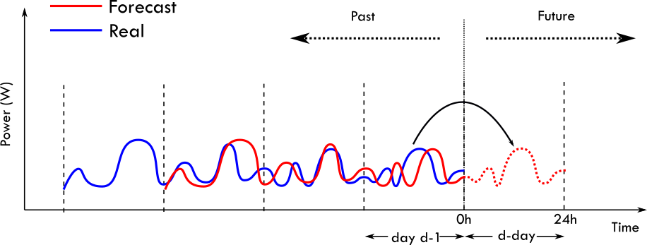
A second method is a naive method, also called persistence. This is obtained using method=naive. This method simply assumes that the forecast for a future period will be equal to the observed values in a past period. The past period is controlled using the parameter delta_forecast_daily and the default value for this is 24h.
This is presented graphically here:
Starting with v0.4.0, a new forecast framework is proposed within EMHASS. It provides a more efficient way to forecast the power load consumption. It is based on the skforecast module that uses scikit-learn regression models considering auto-regression lags as features. The hyperparameter optimization is proposed using Bayesian optimization from the optuna module. To use this change to method=mlforecaster in the configuration.
The API provides fit, predict and tune methods.
The following is an example of a trained model using a KNN regressor:

The naive persistence model performs very well on the 2-day test period, however, is well outperformed by the KNN regressor when back-testing on the complete training set (10 months of 30-minute time step data).
The hyperparameter tuning using Bayesian optimization improves the bare KNN regressor from \(R^2=0.59\) to \(R^2=0.75\). The optimized number of lags is \(48\).
See the machine learning forecaster section for more details.
Load forecast calibration#
With three load forecast methods available (naive, typical and mlforecaster), it is not always obvious which one tracks your own consumption best. The forecast-calibration action produces an on-demand accuracy report to help you pick. It is reporting only: it does not change any optimization and it saves no model or file.
The action retrieves your recent load history (90 days by default, since the typical method needs a long window to be meaningful), splits it chronologically into three windows (train / test / val) and scores every method with a day-ahead walk-forward. To predict a given day, a method may only see history strictly before that day, so there is no look-ahead. The report is shown in the add-on web UI as a graph (actual load versus each method over the validation window) and a metrics table (MAE, RMSE, R2, MAPE, a persistence skill score and the sample count n, per method and per split).
You can launch it from the add-on web UI with the Load forecast calibration button on the advanced page, or over the REST API with an empty body:
curl -i -H 'Content-Type:application/json' -X POST -d '{}' http://localhost:5000/action/forecast-calibration
The three day windows are optional runtime parameters, so you can trade report length against how far back it looks without editing any config. They default to the values above when omitted:
calibration_days_to_retrieve: how much history to pull (default90). Lower it for a quicker run or raise it to cover more of the year. If it is too short for the split below, the action returns a clear “not enough history” message instead of a report.calibration_test_days: size of the held-outtestwindow in days (default14).calibration_val_days: size of the held-outvalwindow in days (default14).
curl -i -H 'Content-Type:application/json' -X POST \
  -d '{"calibration_days_to_retrieve": 120, "calibration_test_days": 21, "calibration_val_days": 21}' \
  http://localhost:5000/action/forecast-calibration
A few things to keep in mind when reading the report:
The
naiveandtypicalmethods have no fitting step, so theirtraincolumn is reported asN/A. Thetraincolumn is an in-sample score formlforecasteronly.The skill score is
1 - method_MAE / naive_MAE, computed over the days a method andnaiveboth cover so the comparison is fair even when a method covers fewer days.naiveis the baseline at0and a positive value means the method beats naive persistence.mlforecasteris fitted fresh in memory on thetrainwindow for this report using a fast LinearRegression baseline; it never reads a model you previously trained withforecast-model-fit, so the report works even if you have never run a fit (and it will not stall on a slow configured estimator).typicalhere is derived from the retrieved history window rather than the long-term typical profile used in production, and it needs prior same-month, same-weekday history, so on a short window it may cover fewer days than the other methods (compare thencolumns).
Load cost forecast#
The default method for load cost forecast is defined for a peak and non-peak hours contract type. This is obtained using method=hp_hc_periods.
Per-deferrable-load cost overrides (hybrid heating)#
By default, every deferrable load is priced at the shared load_cost_forecast (the electricity tariff). For hybrid heating setups - where one deferrable load runs on a different commodity than another (e.g. a heat pump on electricity and a gas boiler on gas) - the shared cost track is wrong: it would dispatch both loads as if they cost the same per kWh.
To handle this, EMHASS supports an optional cost_forecast_per_deferrable_load parameter in optim_conf. It’s a list with one entry per deferrable load:
null(orNone) for a load → keep the sharedload_cost_forecast(default).A list of floats (length equal to the forecast horizon, units
Currency/kWh) → price that load at its own per-timestep rate.
Example: heat pump on deferrable0 keeps the electricity tariff; gas boiler on deferrable1 is priced against a flat gas rate of 0.085 €/kWh:
{
  "cost_forecast_per_deferrable_load": [
    null,
    [0.085, 0.085, 0.085, ...]
  ]
}
The objective adds an adjustment term (per_load_cost - load_cost) * p_deferrable[k] for each load with an override. When the override is unset the adjustment is identically zero, so existing setups are unaffected.
Note: this parameter only adjusts the cost in the objective; it does NOT remove a non-electric load from the electric power-balance constraint. For a gas boiler load, configure nominal_power_of_deferrable_loads[k] in the gas-input units you want the optimizer to dispatch, and exclude that load from the household electric load_forecast so the grid balance reflects only true electric demand.
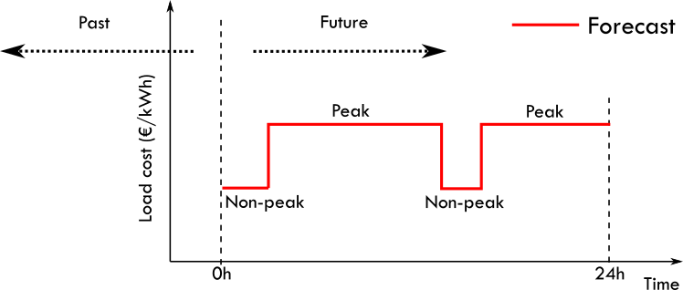
When using this method you can provide a list of peak-hour periods, so you can add as many peak-hour periods as possible.
As an example for a two peak-hour periods contract you will need to define the following list in the configuration file:
- load_peak_hour_periods:
    - period_hp_1:
        - start: '02:54'
        - end: '15:24'
    - period_hp_2:
        - start: '17:24'
        - end: '20:24'
- load_peak_hours_cost: 0.1907
- load_offpeak_hours_cost: 0.1419
This example is presented graphically here:
PV production selling price forecast#
The default method for this forecast is simply a constant value. This can be obtained using method=constant.
Then you will need to define the photovoltaic_production_sell_price variable to provide the correct price for energy injected to the grid from excess PV production in currency/kWh.
Passing your own forecast data#
For all the needed forecasts in EMHASS, two other methods allow the user to provide their own forecast value. This may be used to provide a forecast provided by a more powerful and accurate forecaster. The two methods are: csv and list.
For the csv method you should push a csv file to the data folder. The CSV file should contain no header and the timestamped data should have the following format:
2021-04-29 00:00:00+00:00,287.07
2021-04-29 00:30:00+00:00,274.27
2021-04-29 01:00:00+00:00,243.38
...
For the list method, you just have to add the data as a list of values to a data dictionary during the call to emhass using the runtimeparams option.
The possible dictionary keys to pass data are:
pv_power_forecastfor the PV power production forecast.load_power_forecastfor the Load power forecast.load_cost_forecastfor the Load cost forecast.prod_price_forecastfor the PV production selling price forecast.
For example, if using the add-on or the docker method, you can pass this data as a list of values to the data dictionary during the curl POST:
curl -i -H "Content-Type: application/json" -X POST -d '{
	"pv_power_forecast":[0, 0, 0, 0, 0, 0, 0, 0, 0, 0, 0, 0, 0, 0, 0, 0, 70, 141.22, 246.18, 513.5, 753.27, 1049.89, 1797.93, 1697.3, 3078.93, 1164.33, 1046.68, 1559.1, 2091.26, 1556.76, 1166.73, 1516.63, 1391.13, 1720.13, 820.75, 804.41, 251.63, 79.25, 0, 0, 0, 0, 0, 0, 0, 0, 0, 0]
}' http://localhost:5000/action/dayahead-optim
You need to be careful here to send the correct amount of data on this list, the correct length. For example, if the data time step is defined as 1 hour and you are performing a day-ahead optimization, then this list length should be 24 data points.
Understanding forecast data formats: List vs Dictionary#
EMHASS supports two formats for passing forecast data as runtime parameters: list format and dictionary format with timestamps. Understanding when to use each format can significantly simplify your Home Assistant automations.
List Format (Traditional)#
The list format passes forecast values as a simple array. This is the most compact format but requires careful attention to timing and data length.
Requirements:
The list must contain values for the current time period first, followed by future values
The list length must match your prediction horizon based on
optimization_time_stepValues must be in the correct order (chronological)
Example:
curl -i -H "Content-Type: application/json" -X POST -d '{
	"load_cost_forecast": [0.25, 0.24, 0.23, 0.26, 0.28, ...],
	"prediction_horizon": 24,
	"optimization_time_step": 60
}' http://localhost:5000/action/dayahead-optim
For a 24-hour forecast with 1-hour intervals, you need exactly 24 values starting from the current hour.
When to use list format:
Your forecast data is already aligned with EMHASS intervals
You want minimal JSON payload size
You generate forecast values programmatically in the correct interval
Dictionary Format with Timestamps (Recommended for most users)
The dictionary format allows you to pass forecast values with explicit timestamps. EMHASS will automatically handle resampling, alignment, and gap filling.
Advantages:
Automatic resampling: If your data is hourly but EMHASS runs at 15-minute intervals, resampling happens automatically
Flexible timing: No need to calculate exact list length or worry about current time alignment
Self-documenting: Timestamps make it clear which value applies when
Automatic gap filling: Missing timestamps are filled using forward-fill and backward-fill
Timezone aware: Timestamps are parsed and converted to your configured timezone
Format:
{
	"load_cost_forecast": {
		"2025-10-16 10:00:00+00:00": 0.25,
		"2025-10-16 11:00:00+00:00": 0.28,
		"2025-10-16 12:00:00+00:00": 0.23
	}
}
Example curl command:
curl -i -H "Content-Type: application/json" -X POST -d '{
	"load_cost_forecast": {
		"2025-10-16 10:00:00+00:00": 0.25,
		"2025-10-16 11:00:00+00:00": 0.28,
		"2025-10-16 12:00:00+00:00": 0.23
	},
	"prediction_horizon": 48,
	"optimization_time_step": 15
}' http://localhost:5000/action/naive-mpc-optim
What happens internally:
Timestamps are parsed as ISO8601 format with timezone
Data is resampled to match your optimization_time_step (e.g., from 1h to 15min intervals)
Values are aligned with the forecast horizon using nearest-neighbor interpolation
Any missing values are filled using forward-fill then backward-fill
The result is converted to a list for the optimizer
When to use dictionary format:
Your price data comes from an API (Nordpool, ENTSO-E, Amber, etc.) that provides hourly prices
You want EMHASS to handle interval conversion automatically
Your optimization_time_step differs from your data resolution
You want more readable and maintainable Home Assistant templates
Practical Home Assistant Examples
Dictionary format with Nordpool (Simple - Recommended!):
shell_command:
	emhass_dayahead_nordpool: >
		curl -i -H "Content-Type: application/json" -X POST -d '{
			"load_cost_forecast": {{ state_attr("sensor.nordpool_kwh_be_eur_3_10_025", "raw_today") | tojson }},
			"prod_price_forecast": {{ state_attr("sensor.nordpool_kwh_be_eur_3_10_025", "raw_today") | tojson }}
		}' http://localhost:5000/action/dayahead-optim
The Nordpool integration already provides data in dictionary format with timestamps, so you can pass it directly using | tojson!
List format with Nordpool (Traditional - More Complex):
shell_command:
	emhass_dayahead_nordpool_list: >
		curl -i -H "Content-Type: application/json" -X POST -d '{
			"load_cost_forecast": {{(
				([states("sensor.nordpool_kwh_be_eur_3_10_025")|float(0)] +
				state_attr("sensor.nordpool_kwh_be_eur_3_10_025", "raw_today") | map(attribute="value") | list +
				state_attr("sensor.nordpool_kwh_be_eur_3_10_025", "raw_tomorrow") | map(attribute="value") | list)
				[now().hour:][:24]
			)}}
		}' http://localhost:5000/action/dayahead-optim
Notice how the list format requires:
Adding the current hour value first
[states("sensor.nordpool...")]Extracting values from dictionaries
map(attribute="value")Slicing from current hour
[now().hour:]Limiting to the correct length
[:24]
Dictionary format handles all of this automatically!
Important Notes
Timezone handling:
Timestamps should include timezone information (e.g., +00:00 for UTC, +02:00 for CEST)
EMHASS will convert timestamps to your configured timezone from
secrets_emhass.yamlIf timestamps don’t include timezone, they’re assumed to be in your local timezone
Data resolution:
Dictionary format works best when your source data is at a coarser resolution than your optimization_time_step
Example: Hourly price data automatically resampled to 15-minute intervals
The resampling uses “nearest neighbor” method, so hourly prices are held constant for all 15-minute intervals within that hour
Current values:
When using list format, the first value in the list must be the current period
Example: If it’s 14:30 and your intervals are 30 minutes, the first value should be for 14:30-15:00
Dictionary format automatically handles this by using timestamps
Mixing formats:
You can use list format for some forecasts and dictionary format for others in the same API call
Example:
pv_power_forecastas list,load_cost_forecastas dictionary
curl -i -H "Content-Type: application/json" -X POST -d '{
	"pv_power_forecast": [0, 0, 50, 150, 300, ...],
	"load_cost_forecast": {
		"2025-10-16 10:00:00+00:00": 0.25,
		"2025-10-16 11:00:00+00:00": 0.28
	}
}' http://localhost:5000/action/naive-mpc-optim
Summary: Which Format Should I Use?
Scenario |
Recommended Format |
Reason |
|---|---|---|
Using Nordpool/ENTSO-E/Amber price APIs |
Dictionary |
Data already includes timestamps |
Data from Home Assistant sensors with attributes |
Dictionary |
Easier template syntax |
Hourly data with 15-min optimization intervals |
Dictionary |
Automatic resampling |
Self-generated forecast in Python/Node-RED |
Either |
Choose based on convenience |
Minimal network payload needed |
List |
More compact JSON |
Generated forecast already matches intervals |
List |
No conversion needed |
For most Home Assistant users: Use dictionary format with timestamps for simpler, more maintainable automations.
Example using: Solcast forecast + Amber prices#
If you’re using Solcast then you can define the following sensors in your system:
sensors:

  - platform: rest
    name: "Solcast Forecast Data"
    json_attributes:
      - forecasts
    resource: https://api.solcast.com.au/rooftop_sites/yyyy/forecasts?format=json&api_key=xxx&hours=24
    method: GET
    value_template: "{{ (value_json.forecasts[0].pv_estimate)|round(2) }}"
    unit_of_measurement: "kW"
    device_class: power
    scan_interval: 8000
    force_update: true

  - platform: template
    sensors:
      solcast_24hrs_forecast :
        value_template: >-
          {%- set power = state_attr('sensor.solcast_forecast_data', 'forecasts') | map(attribute='pv_estimate') | list %}
          {%- set values_all = namespace(all=[]) %}
          {% for i in range(power | length) %}
           {%- set v = (power[i] | float |multiply(1000) ) | int(0) %}
            {%- set values_all.all = values_all.all + [ v ] %}
          {%- endfor %} {{ (values_all.all)[:48] }}
With this, you can now feed this Solcast forecast to EMHASS along with the mapping of the Amber prices.
An MPC call may look like this for 4 deferrable loads:
    post_mpc_optim_solcast: "curl -i -H \"Content-Type: application/json\" -X POST -d '{\"load_cost_forecast\":{{(
          ([states('sensor.amber_general_price')|float(0)] +
          state_attr('sensor.amber_general_forecast', 'forecasts') |map(attribute='per_kwh')|list)[:48])
          }}, \"prod_price_forecast\":{{(
          ([states('sensor.amber_feed_in_price')|float(0)] +
          state_attr('sensor.amber_feed_in_forecast', 'forecasts')|map(attribute='per_kwh')|list)[:48])
          }}, \"pv_power_forecast\":{{states('sensor.solcast_24hrs_forecast')
          }}, \"prediction_horizon\":48,\"soc_init\":{{(states('sensor.powerwall_charge')|float(0))/100
          }},\"soc_final\":0.05,\"operating_hours_of_each_deferrable_load\":[2,0,0,0]}' http://localhost:5000/action/naive-mpc-optim"
Thanks to @purcell_labs for this example configuration.
Example combining multiple Solcast configurations#
If you have multiple rooftops, for example for east-west facing solar panels, then you will need to fuze the sensors providing the different forecasts on a single one using templates in Home Assistant. Then feed that single sensor data passing the data as a list when calling the shell command.
Here is a sample configuration to achieve this, thanks to @gieljnssns for sharing.
The two sensors using rest sensors:
- platform: rest
  name: "Solcast Forecast huis"
  json_attributes:
    - forecasts
  resource: https://api.solcast.com.au/rooftop_sites/xxxxxxxxxxc/forecasts?format=json&api_key=xxxxxxxxx&hours=24
  method: GET
  value_template: "{{ (value_json.forecasts[0].pv_estimate)|round(2) }}"
  unit_of_measurement: "kW"
  device_class: power
  scan_interval: 86400
  force_update: true

- platform: rest
  name: "Solcast Forecast garage"
  json_attributes:
    - forecasts
  resource: https://api.solcast.com.au/rooftop_sites/xxxxxxxxxxc/forecasts?format=json&api_key=xxxxxxxxx&hours=24
  method: GET
  value_template: "{{ (value_json.forecasts[0].pv_estimate)|round(2) }}"
  unit_of_measurement: "kW"
  device_class: power
  scan_interval: 86400
  force_update: true
Then two templates, one for each sensor:
    solcast_24hrs_forecast_garage:
      value_template: >-
        {%- set power = state_attr('sensor.solcast_forecast_garage', 'forecasts') | map(attribute='pv_estimate') | list %}
        {%- set values_all = namespace(all=[]) %}
        {% for i in range(power | length) %}
          {%- set v = (power[i] | float |multiply(1000) ) | int(0) %}
          {%- set values_all.all = values_all.all + [ v ] %}
        {%- endfor %} {{ (values_all.all)[:48] }}

    solcast_24hrs_forecast_huis:
      value_template: >-
        {%- set power = state_attr('sensor.solcast_forecast_huis', 'forecasts') | map(attribute='pv_estimate') | list %}
        {%- set values_all = namespace(all=[]) %}
        {% for i in range(power | length) %}
          {%- set v = (power[i] | float |multiply(1000) ) | int(0) %}
          {%- set values_all.all = values_all.all + [ v ] %}
        {%- endfor %} {{ (values_all.all)[:48] }}
And the fusion of the two sensors:
    solcast_24hrs_forecast:
      value_template: >-
        {% set a = states("sensor.solcast_24hrs_forecast_garage")[1:-1].split(',') | map('int') | list %}
        {% set b = states("sensor.solcast_24hrs_forecast_huis")[1:-1].split(',') | map('int') | list %}
        {% set ns = namespace(items = []) %}
        {% for i in range(a | length) %}
          {% set ns.items = ns.items + [ a[i]  + b[i]  ] %}
        {% endfor %}
        {{ ns.items }}
And finally the shell command:
dayahead_optim: "curl -i -H \"Content-Type:application/json\" -X POST -d '{\"pv_power_forecast\":{{states('sensor.solcast_24hrs_forecast')}}}' http://localhost:5001/action/dayahead-optim"
Example using the Nordpool integration#
The Nordpool integration provides spot market electricity prices (consumption and production) for the Nordic, Baltic and part of Western Europe. An integration for Home Assistant can be found here: https://github.com/custom-components/nordpool
After setup the sensors should appear in Home Assistant for raw today and tomorrow values.
The subsequent shell command to concatenate today and tomorrow values can be for example:
shell_command:
  trigger_nordpool_forecast: "curl -i -H \"Content-Type: application/json\" -X POST -d '{\"load_cost_forecast\":{{((state_attr('sensor.nordpool', 'raw_today') | map(attribute='value') | list  + state_attr('sensor.nordpool', 'raw_tomorrow') | map(attribute='value') | list))[now().hour:][:24] }},\"prod_price_forecast\":{{((state_attr('sensor.nordpool', 'raw_today') | map(attribute='value') | list  + state_attr('sensor.nordpool', 'raw_tomorrow') | map(attribute='value') | list))[now().hour:][:24]}}}' http://localhost:5000/action/dayahead-optim"
Now/current values in forecasts#
When implementing MPC applications with high optimization_time_step it can be interesting if, at each MPC iteration, the forecast values are updated with the real now/current values measured from live data. This is useful to improve the accuracy of the short-term forecasts. As shown in some of the references below, mixing with a persistence model makes sense since this type of model performs very well at low temporal resolutions (intra-hour).
A simple integration of current/now values for PV and load forecast is implemented using a mixed one-observation persistence model and the one-step-ahead forecasted values from the current passed method.
This can be represented by the following equation at time \(t=k\):
Where \(P^{mix}_{PV}\) is the mixed power forecast for PV production, \(\hat{P}_{PV}(k)\) is the current first element of the original forecast data, \(P_{PV}(k-1)\) is the now/current value of PV production and \(\alpha\) and \(\beta\) are coefficients that can be fixed to reflect desired dominance of now/current values over the original forecast data or vice-versa.
The alpha and beta values can be passed in the dictionary using the runtimeparams option during the call to emhass. If not passed they will both take the default 0.5 value. These values should be fixed following your own analysis of how much weight you want to put on measured values to be used as the persistence forecast. This will also depend on your fixed optimization time step. As a default, they will be at 0.5, but if you want to give more weight to measured persistence values, then you can try lower \(\alpha\) and rising \(\beta\), for example: alpha=0.25, beta=0.75. After this, you will need to check with the recorded history if these values fit your needs.
References#
E. Lorenz, J. Kuhnert, A. Hammer, D. Heinemann, Photovoltaic (PV) power predictions with PV measurements, satellite data and numerical weather predictions. Presented at CM2E, Energy & Environment Symposium, Martinique, 2014.
Maimouna Diagne, Mathieu David, Philippe Lauret, John Boland, NicolasSchmutz, Review of solar irradiance forecasting methods and a proposition for small-scale insular grids. Renewable and Sustainable Energy Reviews 27 (2013) 65–76.
Bryan Lima, Sercan O. Arik, Nicolas Loeff, Tomas Pfister, Temporal Fusion Transformers for Interpretable Multi-horizon Time Series Forecasting. arXiv:1912.09363v3 [stat.ML] 27 Sep 2020.