Basic system — no PV, two deferrable loads#
Type: Tutorial — learning-oriented, follow step by step.
This is the simplest scenario: no PV installation, two deferrable loads (for example, a water heater and a pool pump). EMHASS schedules when to run each load to minimize cost against the day-ahead electricity price.
System#
Component |
Value |
|---|---|
PV |
none ( |
Battery |
none |
Deferrable load 1 |
water heater, 3000 W |
Deferrable load 2 |
pool pump, 750 W |
Optimization mode |
day-ahead |
Cost function |
profit |
Configuration#
If you are running the EMHASS Add-on, set in the Add-on configuration page:
set_use_pv: false
nominal_power_of_deferrable_loads:
  - 3000
  - 750
operating_hours_of_each_deferrable_load:
  - 5
  - 8
If you are running standalone Docker with config_emhass.yaml, the same keys apply directly.
The values for operating_hours_of_each_deferrable_load are intentional choices for this scenario; the rest of the parameters keep the defaults from config_defaults.json.
Run the optimization#
REST (Add-on or Docker):
curl -i -H "Content-Type: application/json" \
     -X POST -d '{}' \
     http://localhost:5000/action/dayahead-optim
Or use the Add-on action button in the EMHASS web UI: open http://YOUR_HA_IP:5000/, click “Day-ahead optimization”.
For the legacy CLI variant, see Legacy CLI Commands.
Output#
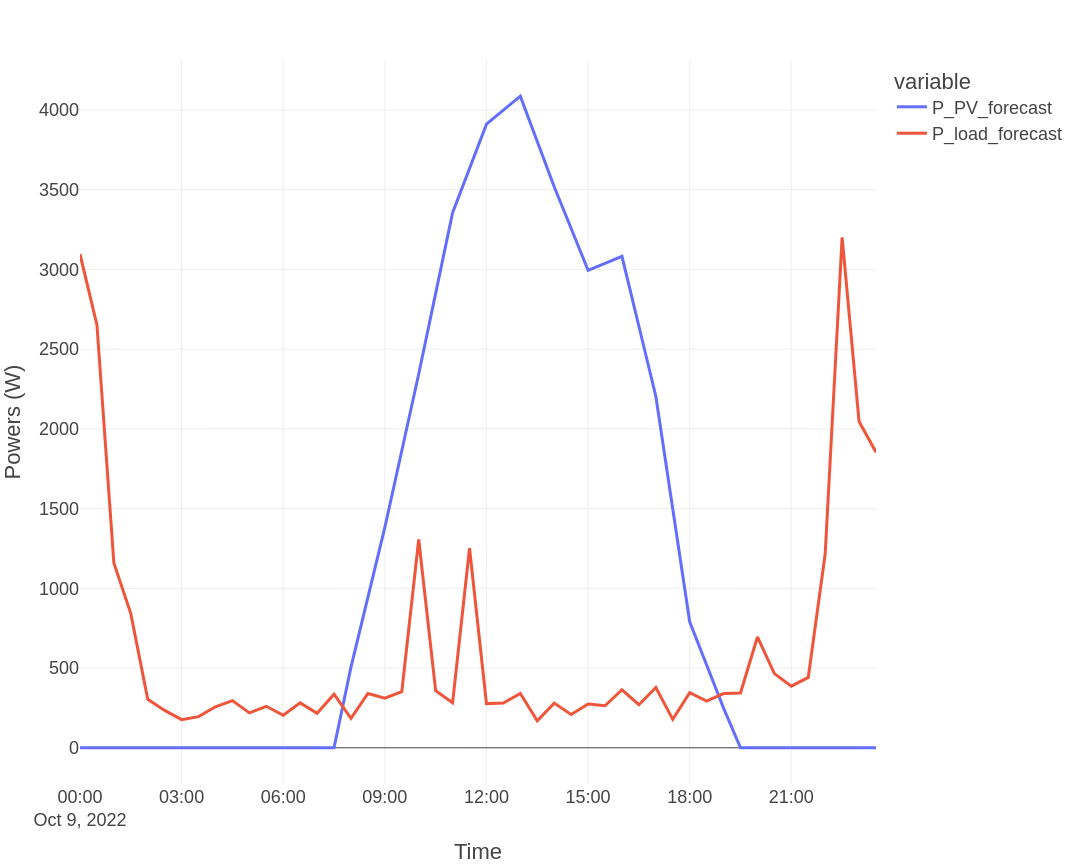
The retrieved input forecasted powers:
The optimization result:
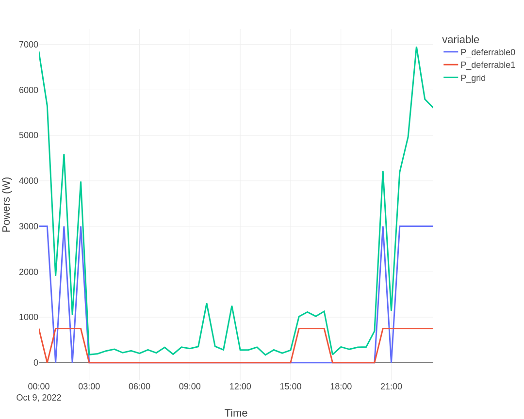
For this system, the total value of the cost function is −5.38 EUR. With costfun: profit, this is net cash flow over the period (positive = revenue, negative = expenditure) — here the system has no revenue source, so the optimizer’s best schedule still costs 5.38 EUR. The schedule places both loads in low-price hours.
Interpretation#
The optimizer treats both deferrable loads as fixed-energy:
load × hours = energy_to_deliver. It is free to choose when in the next 24 h to run them.Without PV, there is no self-consumption opportunity — the only optimization lever is the time-varying load cost.
A cost function of −5.38 EUR for a day with both loads (3 kW × 5 h + 0.75 kW × 8 h = 21 kWh) implies an average paid price of about 0.26 EUR/kWh.
See also#
Tutorial: Basic — PV (same loads + 5 kWp PV)
Reference: Configuration for every parameter
Reference: Passing data for runtime payload schema
How-to: MPC walkthrough when you need rolling-horizon control instead of day-ahead