Basic system — 5 kWp PV, two deferrable loads#
Type: Tutorial — learning-oriented, follow step by step.
This scenario adds a 5 kWp PV installation to the previous tutorial. No battery yet. We run two optimization modes against this system: a 7-day historical perfect optimization (to see what the optimal schedule would have been with hindsight) and a day-ahead optimization (the real production case).
System#
Component |
Value |
|---|---|
PV |
5 kWp |
Battery |
none |
Deferrable load 1 |
water heater, 3000 W |
Deferrable load 2 |
pool pump, 750 W |
Optimization modes |
perfect-optim (backtest), dayahead-optim |
Cost function |
profit |
To enable PV in EMHASS, set set_use_pv: true (default is false) and configure your PV plant via solar_forecast_kwp (for the solar.forecast method) or one of the other weather_forecast_method options. The two deferrable loads use the default nominal_power_of_deferrable_loads: [3000.0, 750.0] from config_defaults.json.
Perfect optimization (7-day historical backtest)#
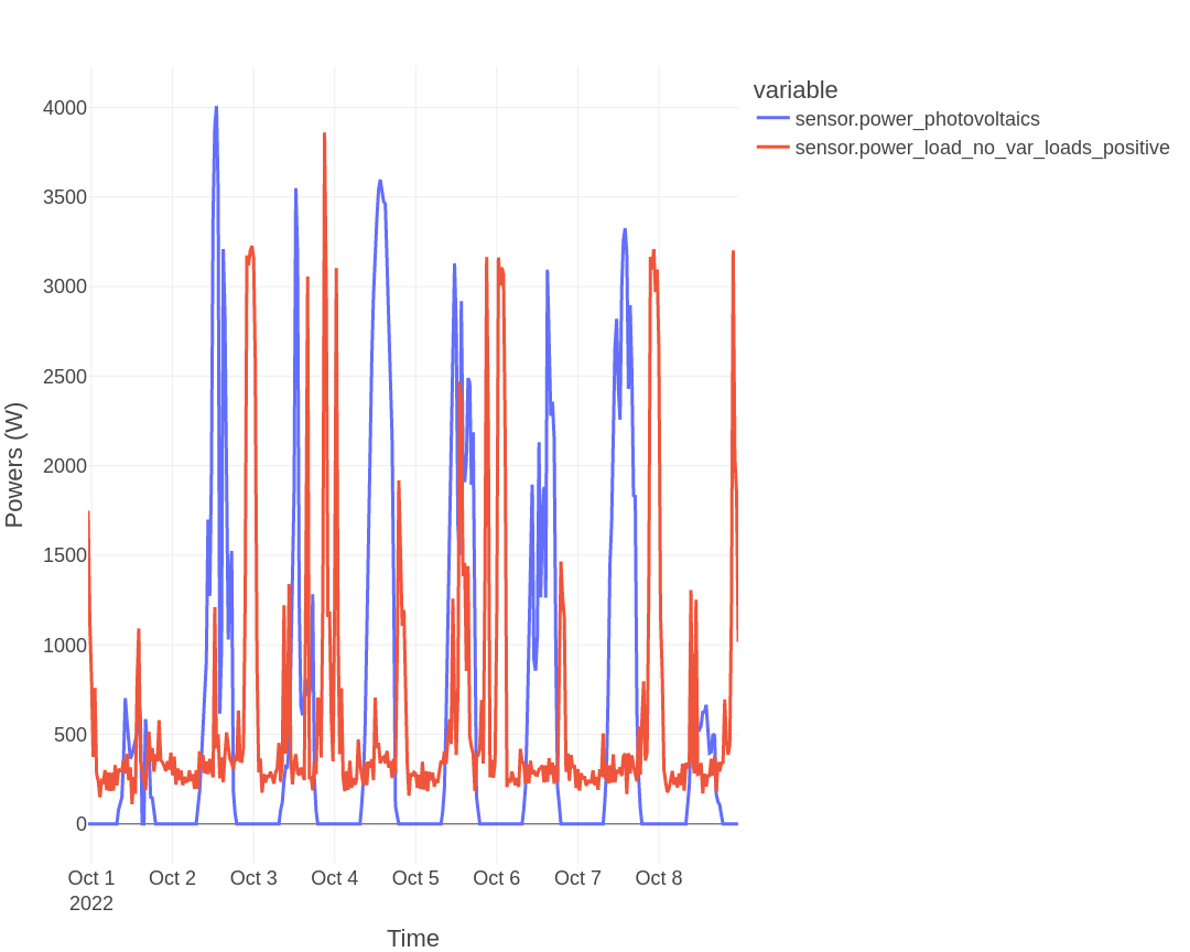
The perfect-optim mode uses real measured PV production and load data from the last 7 days, so the optimizer has perfect knowledge of inputs. The result is the theoretical best-case cost, useful as a benchmark for what dayahead-optim is approaching.
Run it:
curl -i -H "Content-Type: application/json" \
     -X POST -d '{}' \
     http://localhost:5000/action/perfect-optim
Or the Perfect optimization button in the EMHASS web UI.
Inputs (real measured powers over 7 days):
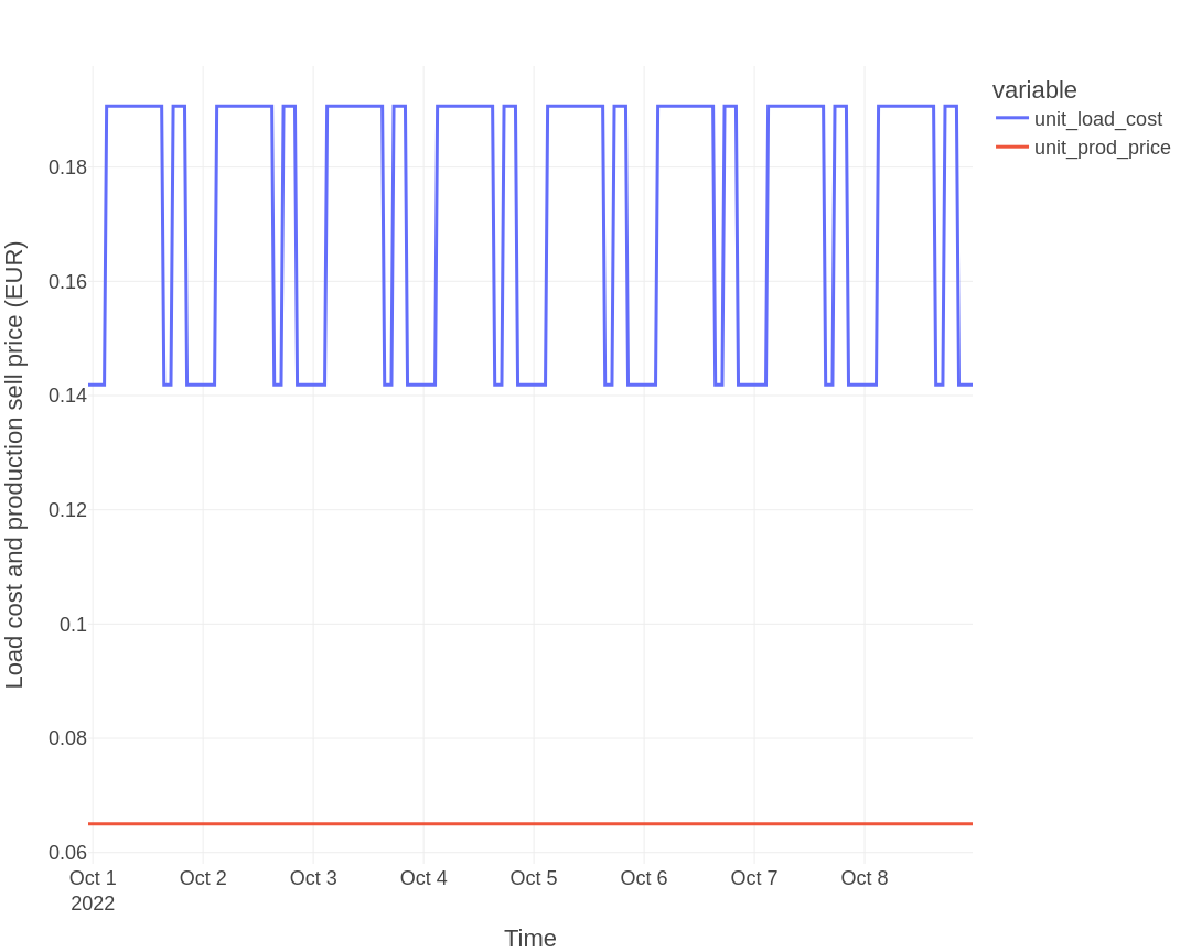
Load cost and PV selling price:
Result:
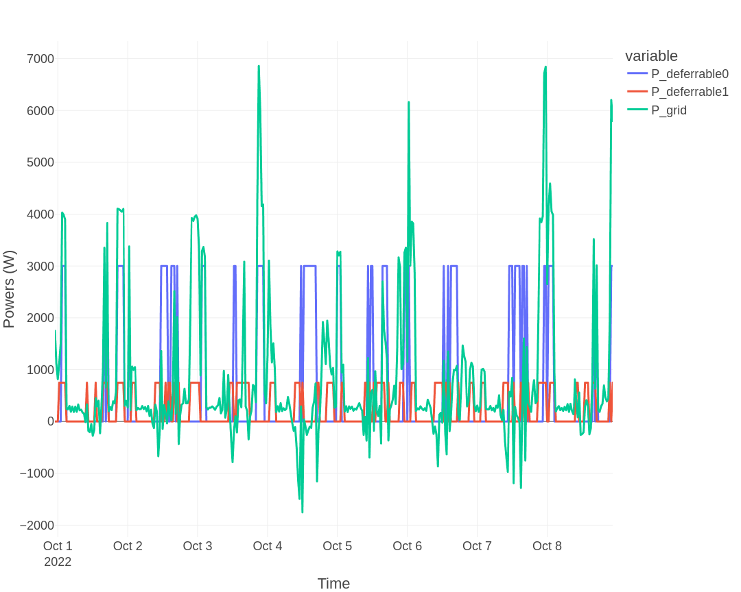
Cost function over the 7-day period: −26.23 EUR.
Day-ahead optimization#
The dayahead-optim mode is the real production case: forecasted PV (from open-meteo by default; alternatives via weather_forecast_method are solcast, solar.forecast, or the scrapper clearoutside method), forecasted load (1-day persistence by default), forecasted prices (provided at runtime if dynamic).
Run it:
curl -i -H "Content-Type: application/json" \
     -X POST -d '{}' \
     http://localhost:5000/action/dayahead-optim
Result:
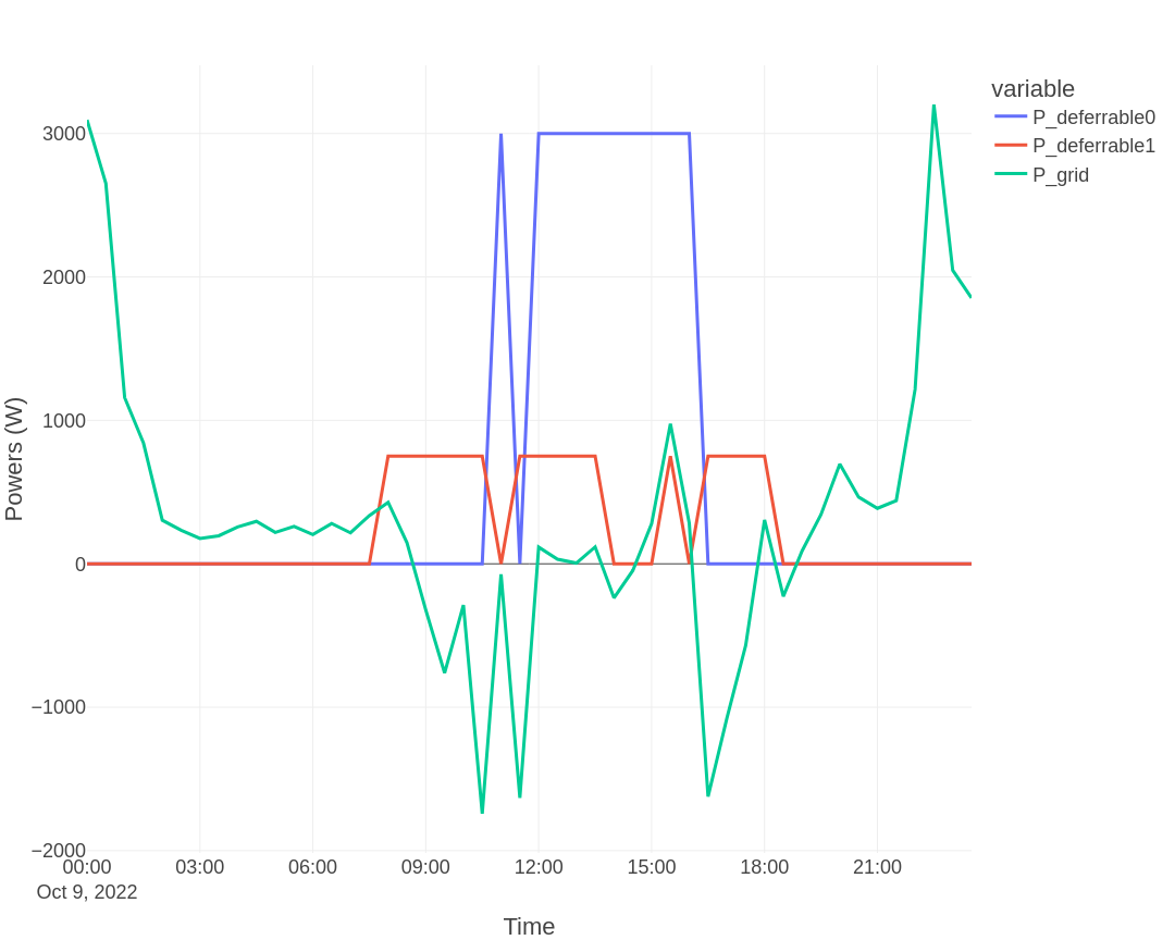
Cost function: −1.56 EUR for the next day. With costfun: profit, this is net cash flow over the period (positive = revenue, negative = expenditure); a less-negative value means lower net cost. Compared with the −5.38 EUR of the no-PV case (see Basic — no PV), the PV installation reduces the daily net spend by about 71%.
Interpretation#
perfect-optim(−26.23 EURover 7 days, ≈ −3.75 EUR/day) gives the theoretical best — the gap todayahead-optim(−1.56 EUR/day) represents forecast uncertainty.The closer your PV-forecast and load-forecast are to reality, the more
dayahead-optimapproachesperfect-optim. Forecast quality is the dominant factor — see Good Practices for details.Without a battery, all PV produced beyond instantaneous load is fed to the grid (or curtailed if
prod_price ≤ 0). Adding a battery typically improves cost further — see the next tutorial.
See also#
Tutorial: Basic — no PV (same loads, no PV)
Tutorial: Basic — PV + Battery (this scenario plus a 5 kWh battery)
Reference: Forecasts for PV/load forecast methods
Explanation: Good Practices for forecast-quality wisdom